Edited: 2020-02-28 07:00:13
Intro
To begin posting interesting statistics tidbits and personal notes online, I first needed to find a suitable workflow to make the publication process as easy as possible. Since I work most days using R with Rstudio, this blogdown-generated site format might just do. Let’s play with it a bit a see what it can do.
For installing etc: https://bookdown.org/yihui/blogdown/
I tweaked the main.css after copying it to static/css; also added a new logo (/static/images/) and favicon (/static/); and other stuff not reported here. In an attempt to be able to have a “front page” I added an /content/index.md but this just messed everything up, so I decided to have this whole blog inside a “blog” folder of main my site root.
Basic features
As far as I can tell, the thing that we can not do with Rmarkdown (rmd) document (as opposed to using md) is todos,
- [x] test maths
- [x] test R blocks
- [x] test biblio
This is of course stated in the reference guide: only md-format supports this, not rmd. The reason is that the formats use different renderer (BlackFriday for md, Pandoc for rmd). But I doubt there is any point making todo-lists on static posts anyway. What else do we have…
Standard lists do work
- first
- jee jee
- joo
- second
- a pina
- b anaani
as do quotations with > symbol
Oli hepokatti maantiellä poikittain.
— somebody
For TOC at the top add to YAML
output:
  blogdown::html_page:
    toc: true
Maths
We are supposed to be able generate posts like we would Rmarkdown-documents, so inline \(\log \xi = a\Rightarrow \xi=e^a\) should work as well as
\[\int_U g(z)dz = G(U)\]
and
\[\begin{align} y_i &= a+ bx_i + z_i\\ z_i &= \varepsilon_i + y_{i-1} \end{align}\]
Hmm direct rendering does seem to work. For the theme hugo-xmin or other similar barebones theme the file layouts/partial/foot_custom.html (or similar) needs a bit of tweaking (see link), mainly need to add the relevant js-inclusions e.g.
<script src="//yihui.org/js/math-code.js"></script>
<script async
src="//cdnjs.cloudflare.com/ajax/libs/mathjax/2.7.5/MathJax.js?config=TeX-MML-AM_CHTML">
</script>
The default theme lithium has the required inclusions by default, providing the math-code.js locally and using MathJax server for the maths.
I decided to install MathJax locally, to avoid future breakage, e.g. here. That particular example might just be a bad copy-paste job, but I keep seeing those unrendered blocks of LaTeX often, especially when opening my own html-rendered Rmd-docs offline.
So to get MathJax working locally on my site, I
- installed mathjax, following their readme.md, by opening a terminal inside the blogdown-site root and running
cd static/js
npm install mathjax@3
mv node_modules/mathjax/es5 mathjax- Modified
themes/hugo-lithium/layouts/partials/footer_mathjax.htmlso that it imports the blogdown-required (or Hugo?) compiler
<script src="/js/mathjax/tex-mml-chtml.js"></script>and now math works even when drafting offline :)
One thing I might need is reference formulas. It seems I can add a tag+label inside the align-environment to show something like \[\begin{align} E\sum_{x\neq y}f(x,y)&=\int f(x,y)\rho^{(2)}(x,y)dxdy \tag{tag 1 is here}\label{eq1}\\ &= Z \label{eq2}\tag{tag 2} \end{align}\] and we can refere to them \(\eqref{eq1}\) and \(\eqref{eq2}\), just put the eqref inside dollars, but it does not have autoincrease.
R chuncks
Basic chunk, no flags
data(iris)
f <- lm(Petal.Width ~ Species, data = iris)
summary(f)
##
## Call:
## lm(formula = Petal.Width ~ Species, data = iris)
##
## Residuals:
## Min 1Q Median 3Q Max
## -0.626 -0.126 -0.026 0.154 0.474
##
## Coefficients:
## Estimate Std. Error t value Pr(>|t|)
## (Intercept) 0.24600 0.02894 8.50 1.96e-14 ***
## Speciesversicolor 1.08000 0.04093 26.39 < 2e-16 ***
## Speciesvirginica 1.78000 0.04093 43.49 < 2e-16 ***
## ---
## Signif. codes: 0 '***' 0.001 '**' 0.01 '*' 0.05 '.' 0.1 ' ' 1
##
## Residual standard error: 0.2047 on 147 degrees of freedom
## Multiple R-squared: 0.9289, Adjusted R-squared: 0.9279
## F-statistic: 960 on 2 and 147 DF, p-value: < 2.2e-16seems to work. How about some graphics, with a caption and caching and message=FALSE to avoid those package loading messages:
library(tidyr)
library(dplyr)
library(ggplot2)
iris %>% group_by(Species) %>%
  gather(quant, value, Sepal.Length:Petal.Width) %>%
  ggplot(aes( Species, value )) + geom_boxplot() + facet_wrap(~quant)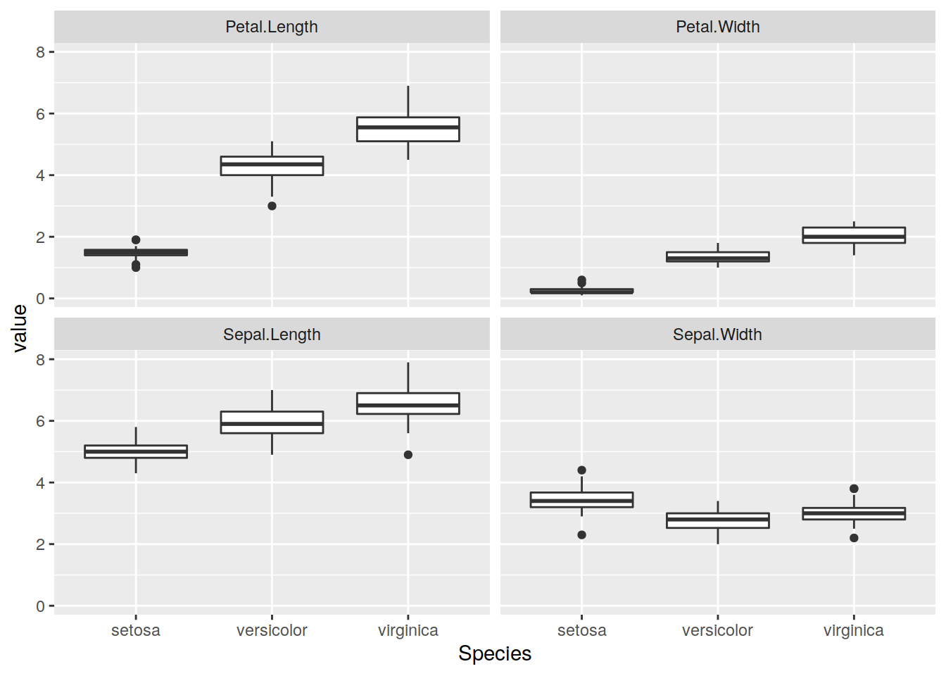
Figure 1: Caption of this figure
Works fine, even adds the “Figure 1” there. Cross-referencing works, see Figures 1 above and 2 below, as long as fig.cap is set.
Try caching for longer runs:
library(spatstat)
pp <- rpoispp(100)
env <- envelope(pp, fun = pcf, verbose = FALSE, divisor="d")
par(mfrow=c(1,2))
plot(pp)
plot(env, ylim = c(0,3))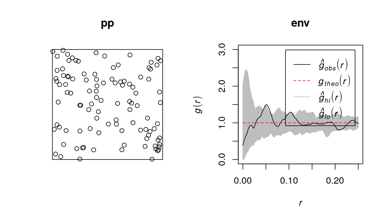
Figure 2: randomness, mot
Seems to work, rendering does not spew out extra messages after the first run.
Citations etc
Simple footnotes work1, just need to write like so2 .
To work with the proper LaTeX-citation system (“BibTeX databases”) I needed to
- Add the bib-files to
content/post, - Install
pandoc-citeproc - Add to the YAML of this Rmd
bibliography: [testbib.bib, testbib2.bib]
link-citations: true
after which we can use the Rmarkdown @-syntax with []-brackets for (),
- Blaa R Core Team (2016); Hynynen et al. (2019)
- Time has come to talk of many things (R Core Team 2016, pp 3-4; also Hynynen et al. 2019 p 1)
Not particularly difficult, and looks quite nice. Just remember to add an empty section-header at the end for the references to have their own space. Note that the footnotes appear below the references. More info on here.
Misc
Images
Another feature that will be needed is static images import and placement. According to the bookdown-book3 we need to envoce the knitr::include_graphics R-call for this, to get this lovely gif included:
knitr::include_graphics("/blog/images/edml915_1232.gif")
Figure 3: Example of a 3D point pattern.
Just remember to store the images in static/images.
Interactive stuff
The above gif is nice visualisation, but an interactive version would be nicer so the reader can spin the data at will. There are many packages for embedding interactive plots in Rmd, e.g. plotly, ggvis, iplot. Example:
library(plotly)
x <- data.frame( sapply(1:3, function(...) runif (n = 1000, min =0, max =1) ),
                 sample(1:2, 1000, TRUE) )
colnames(x) <- c("x", "y", "z", "mark")
x %>% plot_ly(x=~x, y=~y, z=~z,
              color=~factor(mark),
              colors = c("black","blue"),
              type = "scatter3d",
              size = 0.05, alpha=1)
Figure 4: Interactive 3d cloud.
References
Hynynen, Jari, Kalle Eerikäinen, Harri Mäkinen, and Sauli Valkonen. 2019. “Growth Response to Cuttings in Norway Spruce Stands Under Even-Aged and Uneven-Aged Management.” Forest Ecology and Management 437 (April): 314–23. https://doi.org/10.1016/j.foreco.2018.12.032.
R Core Team. 2016. R: A Language and Environment for Statistical Computing. Vienna, Austria: R Foundation for Statistical Computing. https://www.R-project.org/.