A quick note on fetching Finland’s natural protection area -data (luonnonsuojeluealueet) from Syke’s servers into R.
Requirements:
library(sf)
library(dplyr)
library(ggplot2)

# Optional: Polygonal Finland for reference. Provide your own.
fin <- st_geometry(  st_as_sf( suomi::finland_polygons$sp_hires  ) )
Task: Compile a set of all natural protected areas in Finland. Use the simple features-format.
Download data
The website for the data is https://www.syke.fi/fi-FI/Avoin_tieto/Paikkatietoaineistot/Ladattavat_paikkatietoaineistot (2020-02-27). The download links are a bit different.
# The target zips
types <- c("eramaa", "valtio", "yksityinen")
urlf <- "http://wwwd3.ymparisto.fi/d3/gis_data/spesific/luonnonsuojelualueet_%s.zip"

paths <- list()
for(ty in types){
  tmp <- tempfile()
  url <- sprintf(urlf, ty)
  download.file(url, tmp)
  unzip(tmp, exdir = path <- paste0(tempdir(),"/", ty))
  paths[[ty]] <- path
}
Then we read the shape-files in, make sure coordinate system is what we want, add an identifier for type of area, and compile:
# Target CRS is ETRS89 \ TM35FIN. The data should already be in that.
crs <- "+init=epsg:3067"
# read the shapes as sf
polyl <- lapply(types, function(ty){
  x <- st_read(paths[[ty]], quiet = TRUE)
  x <- st_transform(x, crs)
  x$suojeluRyhma <- ty
  x
})

# Then rbind
areas <- do.call(rbind, polyl)
We now got a bunch of polys.
dim(areas)## [1] 14282 29format(object.size(areas), "Mb")## [1] "127.2 Mb"Some checks
According to the data all areas are currently active:
table(areas$Olotila)##
## Voimassa
## 14282Some stats:
areas %>% as.data.frame() %>% group_by(suojeluRyhma) %>%
  summarise(mean_area_km2 = mean(Shape_STAr)/1000^2, n = n())
## # A tibble: 3 x 3
## suojeluRyhma mean_area_km2 n
## <chr> <dbl> <int>
## 1 eramaa 1241. 12
## 2 valtio 25.1 800
## 3 yksityinen 0.267 13470Private ones are very small, wilderness massive.
Simplifying is easy with the sf classes:
areass <- st_simplify(areas, dTolerance = 400, preserveTopology = TRUE)
format(object.size(areass), "Mb")
## [1] "22.9 Mb"Example:
plot(st_geometry( areas[1,]), col = 2, border=NA)
plot(st_geometry(areass[1,]), add=T)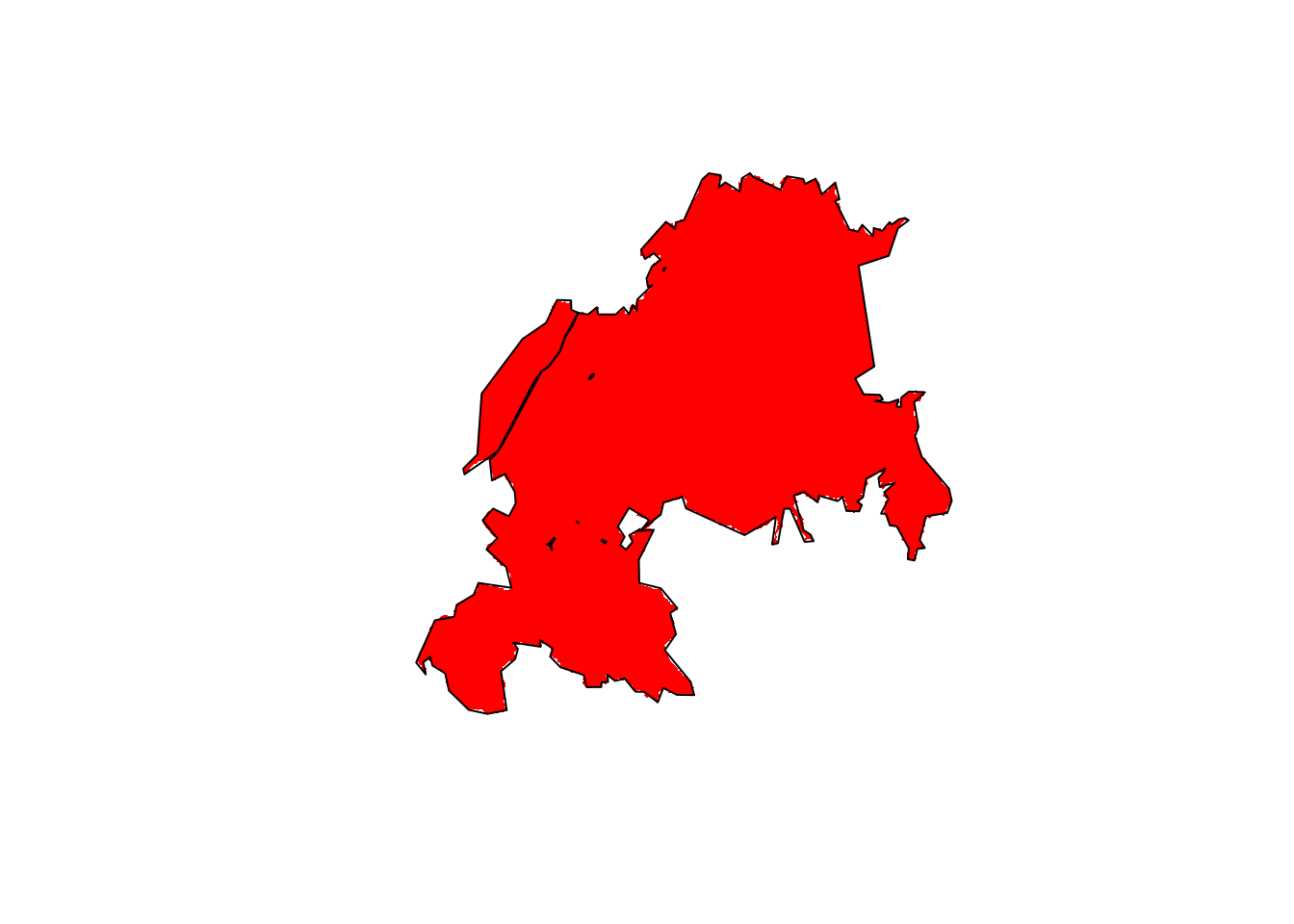
When where the areas established?
According to meta-docs for the files, VoimaantuloPvm should describe when the protection started. But many have filler date with year 9999,
vyears <- format(as.POSIXct( areas$Voimaantul , format = "%Y/%m/%d" ), "%Y")
table(vyears > "2025")
##
## FALSE TRUE
## 2750 11532Let’s assume PaatPvm (date of the decision) is a better starting time. Some are still missing here, though:
pyears <- format(as.POSIXct( areas$PaatPvm, format = "%Y/%m/%d" ), "%Y")
nostart  <- pyears == "9999"
table(paat= nostart, voim=vyears=="9999")
## voim
## paat FALSE TRUE
## FALSE 2750 11492
## TRUE 0 40odd <- st_geometry( areas[ nostart,])
plot(fin)
plot( odd, add = TRUE, col = "red")
plot( st_as_sfc(st_bbox(odd)), add = TRUE)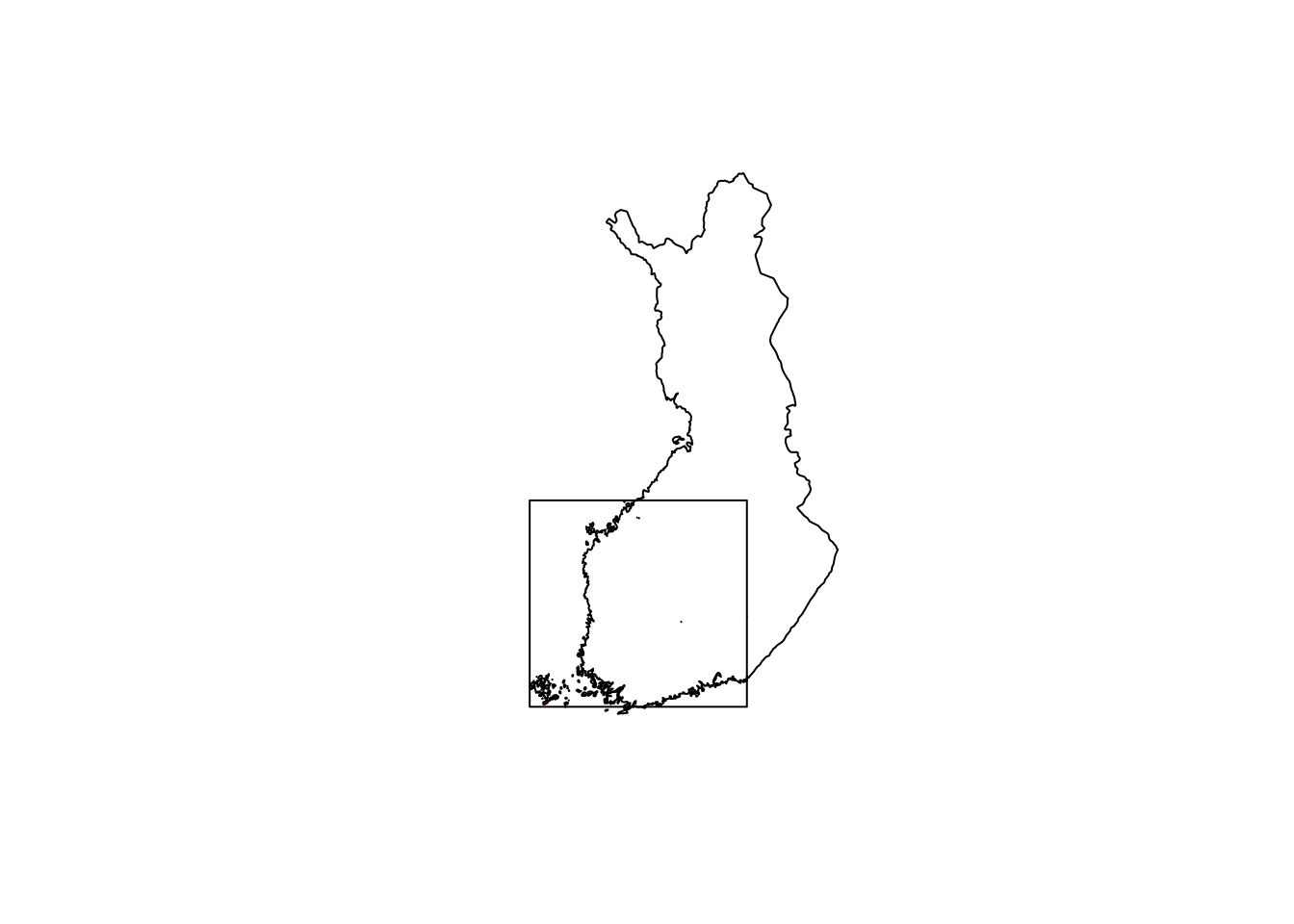
Seems they only exist in Åland area and or are very small. Let’s forget them for now
areas1 <- areass[!nostart,] %>% mutate(start = as.Date( PaatPvm, format = "%Y/%m/%d" ), start_year = format(start, "%Y"))areas1 %>% ggplot() +
geom_histogram(aes(start, fill = suojeluRyhma), position = position_dodge2(width=1)) 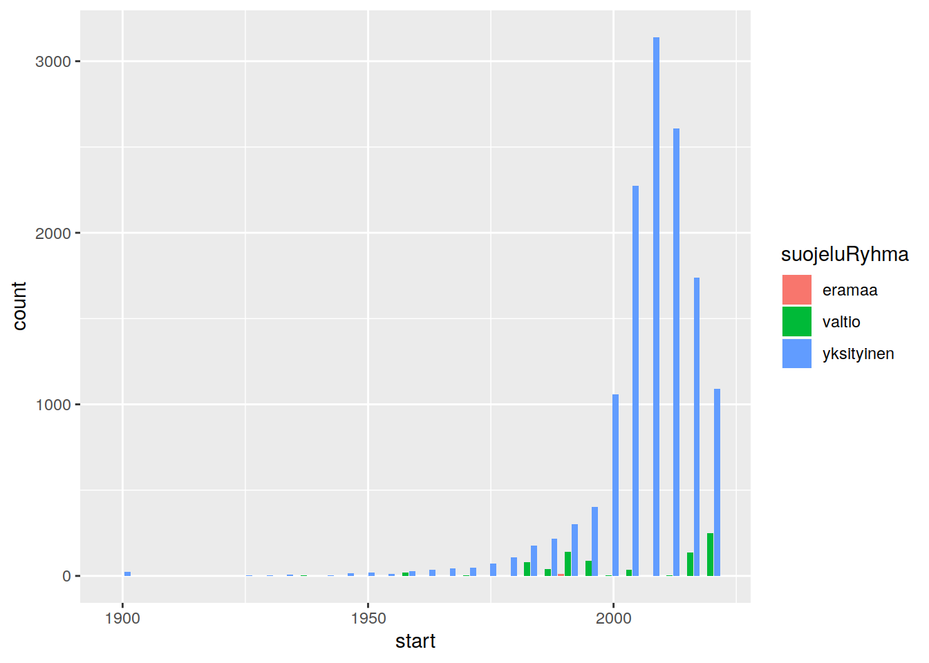
Seems like a lot of private areas have been established since late 1990s.
Area establishment over time
Split by starting time, and plot.
# adhoc groups
areas1 <- areas1 %>% mutate(   start_group =  cut(as.integer(start_year),
                                                  c(0, 1950, 1980, 1990, 2000, 2010, 2020, 2050),
                                                  c("<1950", "1950-1980", "1980s", "1990s", "2000s", "2010s", "2020->"))    )
areas1 %>% ggplot() +
           geom_sf(data = fin, col = "white") +
           geom_sf(aes(fill = suojeluRyhma, col = suojeluRyhma)) +
           facet_wrap(~start_group, nrow=2)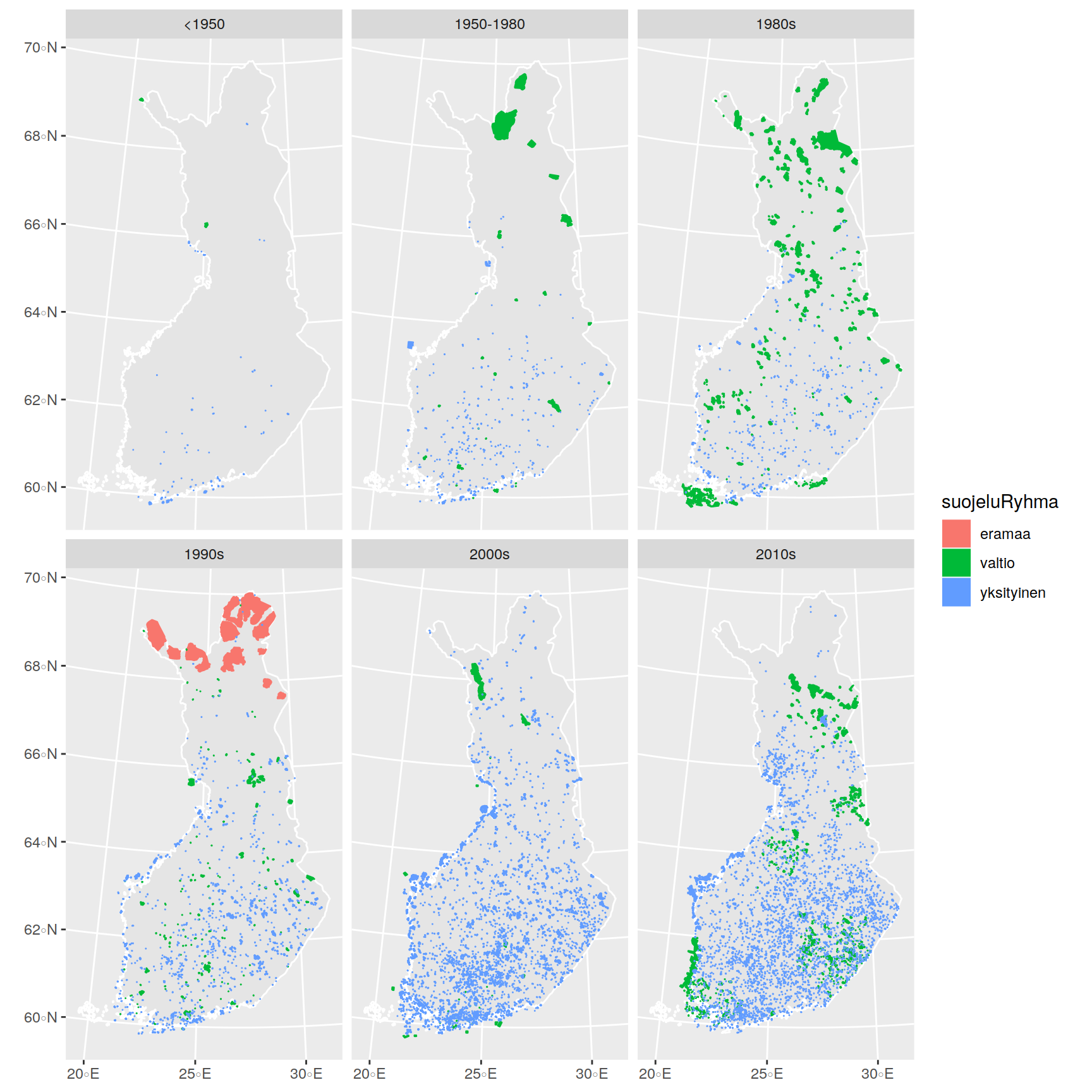
areas1 %>% as.data.frame() %>% group_by(suojeluRyhma, start_group) %>%
  summarise(mean_area_km2 = mean(Shape_STAr)/1000^2, n = n()) %>%
  tidyr::gather(s, v, mean_area_km2:n) %>%
  ggplot(aes(start_group, v, col = suojeluRyhma)) + geom_point() +
  facet_grid(s~suojeluRyhma, scale="free_y") +
  theme(axis.text.x=element_text(angle=45,hjust=1))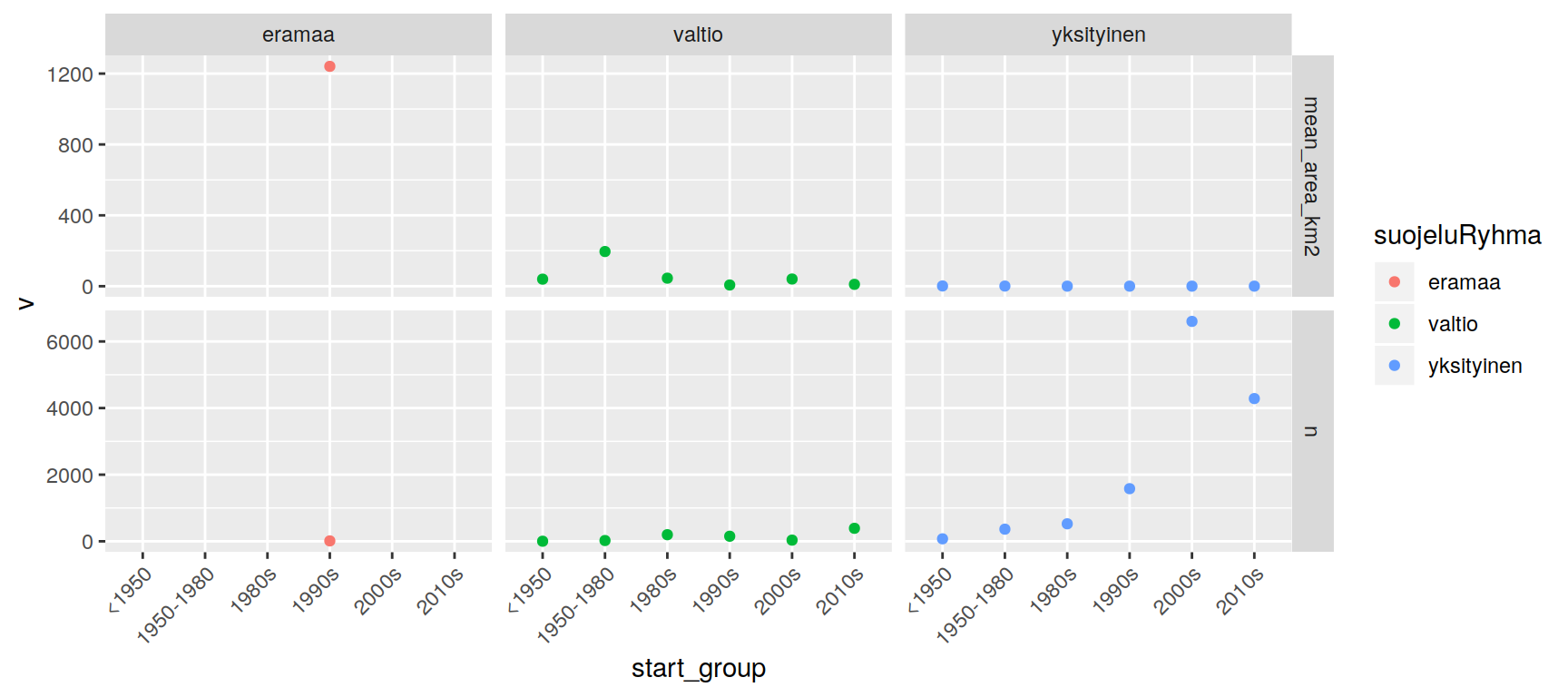
Areas outside mainland
Several areas don’t hit land:
outside <- sapply(st_intersects(areas1, fin) , length) == 0
areasout <- areas1[outside,]
table(as.character( areasout$TyyppiNimi), useNA="i" )
##
## Erityisesti suojeltavan lajin suojelualue (ERA; LsL 47 §)
## 30
## Kansallispuisto
## 3
## Lehtojensuojelualue
## 2
## Luontotyypin suojelualue (LTA; LsL 29 §)
## 135
## Määräaikainen rauhoitusalue (MRA; LsL 25 §)
## 5
## Metsähallituksen päätöksellä perustettu luonnonsuojelu
## 1
## Muu luonnonsuojelualue (MH)
## 33
## Soidensuojelualue
## 1
## Vanhojen metsien suojelualue
## 3
## Yksityismaiden luonnonsuojelualue (YSA)
## 1529Some are special species-protection areas (e.g. seal).